1. Three prediction tasks
Each annotated segment carries three independent labels. We trained separate classifiers for Function (instructional activity), Organization (whole class / groups / individual), and Engagement (All / Most / Half / Some / Not Observable). The same video splits and segment clips were reused; only the target column changed.
2. Data and inputs
- 290 segments from 29 videos with local files (full corpus: 764 segments).
- Per segment: 8 RGB frames (224×224, ImageNet normalization) + mono WAV at 16 kHz.
- Split by video: train 190 / validation 59 / test 41 segments (no segment leakage across splits).
- Written comments on clips were excluded from all reported models (not available at deployment).
- Discussion (Function) and several videos are still off-disk; metrics below apply to the current local subset only.
3. Evaluation metric
Models are scored with macro-averaged F1 (macro-F1): for each class we compute precision and recall, take their harmonic mean (F1), then average across classes with equal weight. Unlike accuracy, macro-F1 does not let the model look good by always predicting the majority class.
We select checkpoints by validation macro-F1 (59 segments). Test (41 segments) is reported but high-variance; we do not use it for model selection.
Training loss vs. macro-F1: macro-F1 is evaluation-only. During training we use a separate loss on the weighted cross-entropy or focal loss (below), with per-class weights in the loss function (weight ∝ 1 / frequency in the training set). That encourages the network to care about rare labels while optimizing gradients; macro-F1 then measures how well that transferred on held-out clips.
4. Four main approaches (used for all three label types)
A. Baseline — video only
- Video: ResNet-18 (ImageNet weights); backbone frozen; 8 frames → mean pool → linear classifier.
- Loss: cross-entropy with class weights (inverse frequency), not focal loss.
- Epochs: 25; AdamW on the trainable head only.
Reference for “frames only, minimal adaptation.”
B. Video v2 — tuned video trunk
- Video: same ResNet-18, but layer3 and layer4 unfrozen (two residual stages) so filters can adapt to classroom scenes.
- Loss: focal loss (γ=2) with the same class weights. Focal loss down-weights easy examples (high-confidence correct predictions) and up-weights hard/minority mistakes in the gradient — this is separate from macro-F1, which is computed only after training on frozen predictions.
- Dropout 0.4 on the head; 20 epochs.
C. Multimodal (mel128) — video + time-warped log-mel
- Video: ResNet-18 with one unfrozen block (layer4), 8-frame mean pool.
- Audio: log-mel spectrogram → resized to fixed 64×128 → small 2-layer CNN → 128-D vector → concat with video → linear classifier.
- Loss: focal loss + class weights; batch size 4; 25 epochs.
See §5 for how mel is computed and why 128 time bins matters.
Why we added approach D after C
Your understanding is correct. Approach C takes a log-mel spectrogram with a variable number of time frames (one column per ~10 ms of audio) and resizes it to a fixed 64×128 grid for every segment. That forces a 3 s clip and an 80 s clip through the same time width, which compresses long speech and stretches short bursts.
Approach D (mel_time) was introduced to test whether preserving the native temporal pattern (same frame rate, no warp to 128 columns) improves performance. We still cap extremely long clips at 512 frames (~5 s of mel frames at our hop size) and pad shorter clips to 512 with a mask, but we no longer squash every segment to identical time geometry before the conv layers. On Function validation, D (0.27) beat C (0.21); on Organization, C and D did not beat video-only baseline.
D. Multimodal (mel_time) — video + native-duration log-mel
- Video: same as B (two unfrozen blocks).
- Audio: log-mel at ~100 frames/s; use the first 512 frames if longer, else pad to 512; mask marks real vs pad frames; 1D conv over time → masked mean pool → 128-D.
- Loss: focal loss + class weights; 20 epochs; features pre-cached under
data/audio_features/mel_time/.
5. Audio encoding (shared pipeline)
5.1 From WAV to log-mel
- Load segment WAV; resample to 16 kHz mono if needed.
- Mel spectrogram:
torchaudio MelSpectrogramwithn_mels=64,n_fft=400,hop_length=160(~10 ms per frame). - Log compression:
log(mel + 1e-9)on power mel (natural log). We always use log-mel for modeling; linear mel power is not fed to the network.
Axis interpretation: vertical = mel frequency bin (64); horizontal = time frame index (depends on clip length).
5.2 Fixed 128-column warp (approach C)
After log-mel, we apply bilinear resize to 64×128 regardless of clip duration. Long clips are compressed along time; short clips are stretched. That was convenient for batching but hurt Function when lectures (~2 min) and directions (~10 s) were forced into the same shape.
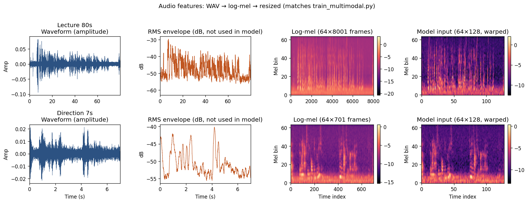
1924 Pre-session.mp4 (open WAVs below).
Columns: waveform → RMS (visualization only) → native log-mel (64×T) → 64×128 warped input to approach C.
Top row: 80 s Lecture; bottom row: 7 s Direction. The warped plot has the same width for both; the long clip loses temporal detail.
Lecture (80 s):
WAV ·
0:00:00–0:01:20 · Function label: Lecture
Direction (7 s):
WAV ·
0:01:20–0:01:27 · Function label: Direction
5.3 Native timing (approach D, mel_time)
After log-mel is computed, we keep one time column per ~10 ms hop (about 100 frames per second of audio). Two cases:
- Clip shorter than ~5.1 s (fewer than 512 mel frames): all frames are kept; the tensor is zero-padded on the right to length 512. The mask is 1 on real frames, 0 on padding.
- Clip longer than ~5.1 s (more than 512 mel frames): we truncate to the first 512 frames only; the mask is 1 throughout (no padding). Audio after that cutoff is not seen by the model.
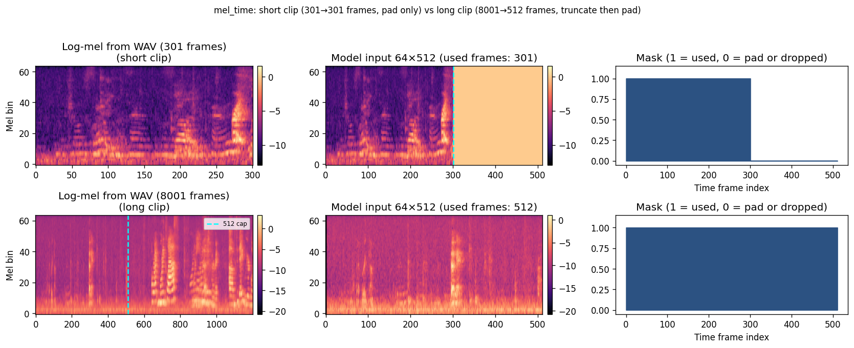
Short example (301 frames, pad only):
1924 Pre-session · 0:27:49–0:27:52 ·
WAV
Long example (8001→512 frames, truncate):
1924 Pre-session · 0:00:00–0:01:20 (Lecture) ·
WAV
5.4 Speech transcription path (Function experiments only)
For the Whisper variant we run whisper-tiny on each WAV, keep the transcript text, then embed it with MiniLM (384-D). The multimodal model concatenates video + embedding. Quality of the pipeline depends on ASR; example for the Lecture clip above:
Annotation comment on that segment: “teacher explaining about input and output.” The transcript is usable but noisy (repetitions, run-on sentences); with only 190 training clips, val/test scores for this branch were unstable.
6. Other audio representations (Function only)
Besides approaches C and D, we ran additional Function experiments. Organization and Engagement used only §4. Validation macro-F1 for these branches is summarized in the muted rows of the §7 Function table; detail below.
Prosody vector (15 numbers) — val 0.10
Instead of a spectrogram image, we summarize the whole WAV with a small set of hand-crafted statistics. No convolution over time-frequency pixels — only these scalars fed to a small MLP:
- Loudness (RMS): average and variability of short-window energy; peak loudness in dB.
- Voice-activity fraction: share of 30 ms windows classified as “speech-like” vs silence/noise (energy-threshold fallback when a dedicated VAD library was unavailable). High values suggest sustained talking.
- Spectral centroid: “brightness” of the sound — where most energy sits on the frequency axis (higher ≈ sharper / less bass-heavy). We store mean and variability across frames.
- Spectral rolloff: frequency below which ~85% of energy lies — another timbre cue (speech vs hum vs crowd).
- Zero-crossing rate: how often the waveform crosses zero; relates to noisiness / frication.
- Speech-segment counts: number of contiguous “voiced” runs, mean/max duration — captures burstiness (many short hits vs one long teacher monologue).
Too coarse to separate Function classes on this dataset.
PANNs embedding (512-D) — val 0.26
PANNs (Pretrained Audio Neural Networks) is a CNN trained on AudioSet to recognize thousands of everyday sound events. We pass each segment WAV through the frozen network and take a 512-dimensional summary vector as the audio input (concatenated with video features). The hope is that “speech,” “applause,” “music,” etc. are partially captured without training a mel-CNN from scratch on 190 segments.
Whisper-tiny + MiniLM (384-D) — val 0.19
Pipeline: (1) Whisper-tiny automatic speech recognition writes an English transcript of the clip; (2) a small sentence encoder (MiniLM) maps that text to a 384-D vector; (3) the classifier uses video + vector. This tests whether what is said carries Function signal. See §5.4 for a transcript example. ASR errors and repetition hurt quality; with small data, validation and test disagreed (test once looked much better by chance).
Annotation comments via TF-IDF — val 0.21 (masked at eval)
Each segment has a short free-text comment in the spreadsheet (e.g. “students working”). We built a bag-of-words representation: count how often each word appears, down-weight words that appear everywhere (TF-IDF). Vocabulary fit on training segments only. At validation/test we feed zeros so scores reflect deployment without comments. A separate “oracle” validation run (true comments injected) scored higher — useful only as a ceiling, not a deployable model.
7. Results (macro-F1)
Validation = model selection; test = held-out videos (small N).
Function
| Approach | Val | Test |
|---|---|---|
| Baseline (video only) | 0.25 | 0.21 |
| Video v2 | 0.26 | 0.34 |
| Multimodal mel128 (§4 C) | 0.21 | 0.22 |
| Multimodal mel_time (§4 D) | 0.27 | 0.20 |
| Other audio inputs (§6) — supplementary; did not beat primary rows on validation | ||
| Prosody vector (15-D) | 0.10 | 0.08 |
| PANNs embedding (512-D) | 0.26 | 0.11 |
| Whisper-tiny + MiniLM (384-D) | 0.19 | 0.35 |
| TF-IDF comments (masked at eval) | 0.21 | 0.16 |
Muted rows are Function-only audio ablations from §6; test scores are noisy (n=41).
Organization
| Approach | Val | Test |
|---|---|---|
| Baseline | 0.42 | 0.31 |
| Video v2 | 0.29 | 0.30 |
| Multimodal mel128 | 0.30 | 0.37 |
| Multimodal mel_time | 0.33 | 0.28 |
Engagement
| Approach | Val | Test |
|---|---|---|
| Baseline | 0.24 | 0.24 |
| Video v2 | 0.25 | 0.19 |
| Multimodal mel128 | 0.27 | 0.15 |
| Multimodal mel_time | 0.30 | 0.11 |
Summary
- Organization is most predictable from video (baseline val 0.42); extra audio did not beat simple frames.
- Function benefits slightly from mel_time on validation; confusions remain between Direction, Transition, and Working.
- Engagement is weakest; mel_time wins validation but test drops sharply (rare classes, n=41 test).
8. Function examples (best val model: mel_time)
Validation clips from mm_mel_time (59 segments). Thumbnail is the first of eight sampled frames;
click to view larger. Comments are annotations only, not model inputs.
Correctly classified (5)
| Frame | Segment | Comment | True | Predicted |
|---|---|---|---|---|
| 1927 · 0:16:44–0:19:29 | Teacher making students st on the carpet and controlling their behaviors | Direction | Direction | |
| 1926 · 0:00:26–0:02:28 | Introduction to BeeBot - Teacher showing a BeeBot on screen and asking questions about its buttons | IRE/MS | IRE/MS | |
| 1926 · 0:02:28–0:04:51 | Teacher playing a video to show kids how a BeeBot works - At this point, whole class was sitting in front of the scre... | Lecture | Lecture | |
| 1924 · 0:03:10–0:04:26 | teacher distributing worksheets and setting up the camera | Transition | Transition | |
| 1924 · 0:28:46–0:31:32 | students working on the lists | Working | Working |
Misclassified (5)
| Frame | Segment | Comment | True | Predicted |
|---|---|---|---|---|
| 1926 · 0:13:02–0:14:16 | Teacher giving directions to students to line up | Direction | Working | |
| 1924 · 0:04:26–0:11:44 | teacher asking questions | IRE/MS | Transition | |
| 1927 · 0:03:08–0:05:56 | Teacher talking about coding | Lecture | Direction | |
| 1927 · 0:14:00–0:16:44 | Teacher distributing tickets and guiding students to their seats | Transition | Direction | |
| 1924 · 0:23:50–0:27:49 | students working together in 2 groups | Working | Transition |
9. What worked and what did not
Worked: video-level splits; log-mel with native timing for Function/Engagement val; Organization from frames alone; focal loss + partial fine-tune for hard Function classes.
Did not: prosody-only vector; fixed 128-bin mel warp for long clips; relying on test F1 (41 clips); comment text at inference; fine-grained Engagement with very few “Half” examples.